The Ising Model and CA, Part II: The Ising CA

October 21, 2025

What is the Ising model CA? How would you attach it to a heat bath?

This is a multipart series. Read the others here:

Aside: I just re-read my older posts and realised how bad I am at writing for an audience made of people other than myself… I am actively going to try and use less jargon from now on…. But unfortunately this series of posts would become wayyy too long if I try writing it for a general audience, so some jargon is inevitable.

Note: while doing the research for writing this post, I stumbled upon this paper: Michael Creutz , “Deterministic Ising Dynamics,” Annals of Physics, 167 (1986) 62-76. What the author tries to do there is actually very similar to what I am doing! They also design a purely deterministic CA to simulate the Ising model. But they seem to have taken a different approach, where instead of having a single giant heat bath separated from the main Ising arena, they couple a tiny heat bath of capacity 3 to each cell. This is actually… a really elegant idea. It requires only 16 states, and there is no need for a separate heat bath. I still feel my method is much more fun, as it seems much more like a physical material, and this allows you to measure a lot of interesting quantities like thermal conductivity, by sandwiching it between two baths, similar to how you would measure it for a real material.

In the last post, we saw how thermodynamics in general works in CA. Now, we will specifically look at the Ising model.

The Ising CA

This one is not actually my invention; it has been explored by some famous names in cellular automata, e.g. see page 4 here. It has two states, ‘up’ and ‘down’. The rules are pretty simple:

We will only update a cell if the following two conditions are met:

$x+y+t$ is even (i.e. the updates follow an alternating chessboard pattern)
The state flips if there are exactly two adjacent up and two adjacent down cells

This conserves energy according to the definition of energy in the Ising model, as the number of adjacent up-down pairs is always constant.

It also happens to be reversible. The reverse rule happens to be itself, with the checkerboard flipped. To see this, what we do is apply the rule without flipping the chessboard pattern. Because of the chessboard pattern, the number of neighbours of a particular colour for each changed cell remains the same, and so the exact same cells get flipped again. Hence, the step gets reversed.

As we know that this rule is both reversible and energy-conserving, we can apply the principles of thermodynamics here.

But, here, a problem is that, unlike the previous case, we cannot assume all the energy locations are independent, so there is no obvious way to determine the temperature. But the same definition still works: The energy needed to increase entropy by one unit.

To actually measure the entropy, there is a known formula, but it is very complicated. And the formula can be found only after you find the exact solution to the model, so I think it’s cheating to use that. That is why, to actually work with temperature, we couple it with a system whose temperature can be easily calculated.

Now, you can use this even without a heat bath to calculate the graph between energy density and magnetisation. Here is approximately how they would look (I got lazy, these are the graphs when it is coupled to the heat bath with slow energy loss, but they should look the same)

E vs m

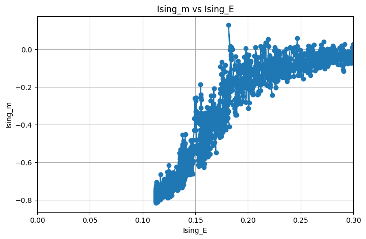
Some observations:

I cut off the graph at low energies. This is because the system starts to get ‘frozen’ and hence energy transfer becomes too slow. So you would have to wait for an impractically long time in order to reach equilibrium.
You see that $|m|$ drops drastically between $E=0.15$ and $E=0.2$ . This is where the phase transition happens!
It is extremely noisy and not smooth. To get a properly smoothed graph, we will have to take multiple samples at each energy level and do some averaging. This is STATISTICAL mechanics, so nothing is absolute; everything is always fluctuating.

It gives the expected results, but the phase transition is not very satisfying to watch. To see a proper one, we will need to move on to designing an interface between our heat bath and our Ising CA.

The Interface

The interface consists of a row of cells that can carry energy both in the form of HPP energy packets and Ising bonds. The big picture idea behind its evolution is very simple: In every step where it is active, it interconverts energy between its Ising form and its gas form. I’ve tried to make this visible through the icons given to each state. The only problem is that we must respect the chessboard update pattern, reversibility, and all the conservation laws.

Proving this manually for every CA transition rule is not easy, as there will be a lot of states because the two CAs have pretty different ways of conserving energy, and this means it is not straightforward for the interface to conserve energy. Hence, to simplify matters, I decided to divide every step of the CA into two substeps:

Energy movement
State permutation

The movement of the HPP gas and the Ising spin flip both happen under step 1. The HPP reflection rule, interface energy transfer and the chessboard alternation all happen under step 2.

By ensuring that both steps satisfy energy conservation and reversibility, we can prove the final rule does so too, which makes enforcing these much simpler.

The proof of reversibility and energy conservation of the first part can be directly copied from the same proofs for HPP and the Ising CA.

For the second step, note that all possible energy transfers are compulsory, so when doing it again, the energy just gets transferred back.

So that is it! The interface has been successfully designed, and now we can move on to analysing the behaviour of the final system in the next post.

The gory details: The Golly Rule format and Nutshell

To actually run the CA, we have to specify it in some standard format. The CA rule format accepted by most CA software is the rule table.

In this format, rules are specified as transitions. For example, the line

0, 0,0,0,0,0,1,1,1, 1

signifies that a 0 cell with exactly three 1 neighbours turns into a 1. It also supports variables, which allow you to compact multiple transitions into one line.

Unfortunately, it is a pain to write manually, so Nutshell was created. Nutshell adds several helpful features, like independent variables and temporary symmetry switching.

While designing the rule, the number of nutshell transitions also turned out to be pretty large (54), so I decided to write a Python script to generate the transitions for me. It also allowed me to properly incorporate the 2 step way of thinking about the rule that I had described. It also makes debugging and iterating much simpler.

So in the end, to generate the rule file, you have to run my code and then copy-paste the output into a template. This template would contain the rule name and the icons for every state. Then we have to compile that using Nutshell. And then paste the output rule file into Golly. Which turns out to be an extremely convoluted workflow….

A lot of the complexity arises because energy conservation and reversibility are not natural concepts in the rule table format. Another complication is that the symmetry obeyed by the HPP gas involves a rotation and a state permutation, so it is not natively supported anywhere. So you have to manually specify all four directions separately.