Exploring AI Model Diversity
Exploring the properties of the different types of models you can get from training.
As a learning exercise, I trained a small model for a simple binary classification task based on cellular automata. The training data for this task can be easily generated using a simple program, yet the features are pretty noisy, which resembles ‘real’ data in a way. This makes it quite nice as a toy problem, and the results I found reveal the huge variety of models that can be found after training, even when using a constant set of hyperparameters.
The specific problem is this: Given a 128x128 board with the ash created from either HighLife or Conway’s Game of Life (CGOL), the model has to figure out which one is which. For context, an average soup from both is given here:
Once everything settles into periodically repeating patterns (could take thousands of steps!), the leftover pattern is called ash. The main differences are the presence of ‘traffic lights’ (those sets of four alternating lines) and ‘honey farms’ (another set of four items) in CGOL and the presence of an unnamed constellation in HighLife ash. There are also differences in the frequencies of the most common patterns. A nice comparison of frequency can be found on Catagolue - Click under root to go to a HighLife haul, CGOL frequency table
At first glance, this is a perfect problem for a CNN to solve. The model I used has a residual pipeline, and it has been designed in a way such that you can pretty easily swap any two layers, if you are careful about the stride and dilation, as I will elaborate later. This allows for a lot of interesting experiments on how the model changes its internal representations. Also, spatial arrangement and exact distances are extremely critical here, so pooling isn’t a good idea. This is the architecture I am going to work with (in PyTorch):
class CAC_layer(nn.Module):
    def __init__(self, C : int, r : int):
        super().__init__()

        self.seq = nn.Sequential(
            nn.BatchNorm2d(C),
            nn.Conv2d(in_channels=C,out_channels=r*C,kernel_size=3,padding=1,stride=2),
            nn.LeakyReLU(),
            nn.Conv2d(in_channels=r*C,out_channels=C,kernel_size=1),
        )

    def forward(self, input_data):
        return self.seq(input_data)

class ResCNN_CAC(nn.Module):
    def __init__(self, W : int, C : int, r : int, d : int):
        super().__init__()

        self.W = W
        self.C = C
        self.r = r
        self.d = d

        self.embed = nn.Sequential(
            nn.Conv2d(in_channels=2,out_channels=C,kernel_size=3,padding=1),
            nn.BatchNorm2d(C),
            nn.LeakyReLU(),
        )

        self.layers = nn.ModuleList([
            CAC_layer(C,r)
            for i in range(d)
        ])

        self.extract = nn.Sequential(
            nn.Conv2d(in_channels=C,out_channels=r*C,kernel_size=1),
            nn.AdaptiveMaxPool2d(1),
            nn.LeakyReLU(),
            nn.Flatten(),
            nn.Linear(in_features=r*C, out_features=1),
        )

        self.lossfn = nn.BCEWithLogitsLoss()

    def forward(self, batch_data : Float[torch.Tensor, "N 2 W W"]):
        x = self.embed(batch_data)

        for i in range(self.d):
            x = x[:,:,::2,::2] + self.layers[i](x)

        return self.extract(x).squeeze(-1)
I discovered that this model exhibits a very interesting phenomenon: after a good number of batches of training, when the loss has dropped to approximately 0.4, different training runs diverge in their behaviour. Normal metrics like loss, test loss and error rate decrease normally with no notable difference from run to run, but in a lot of runs, ‘swapped metrics’ (loss and error when the last two layers are swapped) seemed to start climbing after this critical point rather than falling with loss.
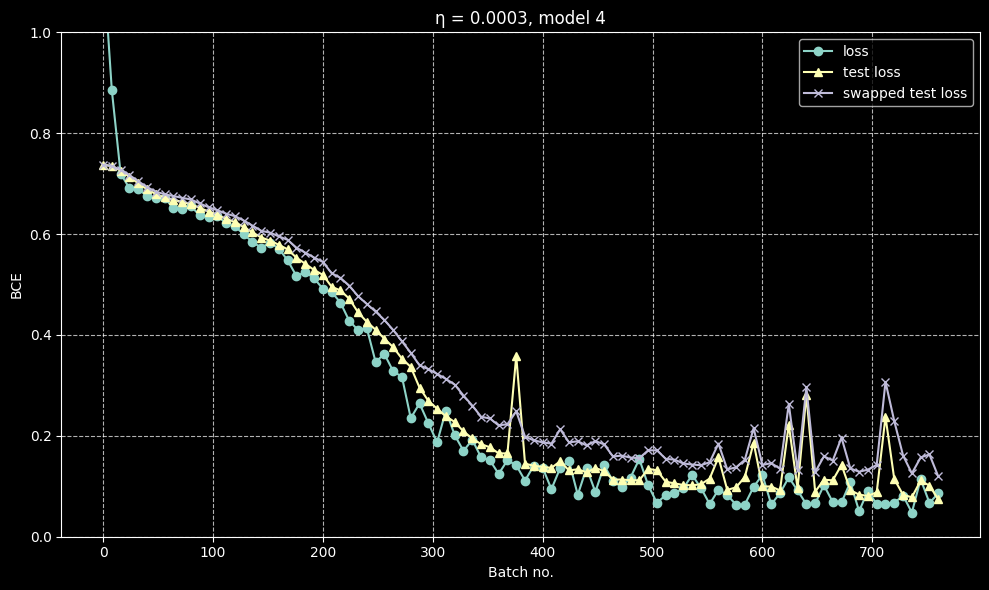 A case where they are about the same
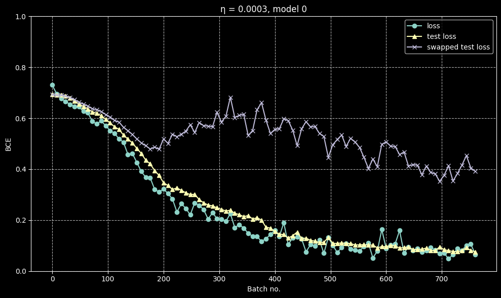 A case where they diverge
I trained 128 different models on the same data, but with the same hyperparameters. I then chose five of the models which degraded the least under swap and five of the ones that degraded the most for further analysis. Initially, I thought the models formed a binary, but further testing has shown that there is a wide variety of behaviours within each group itself, and swap loss itself forms a smeared spectrum. It is interesting that the other two things I tried, SAE and linear probing, did not have their results correlate much with swap loss.
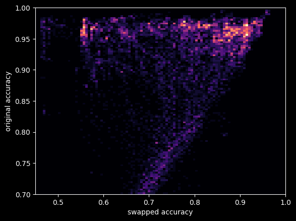
This is a heatmap for (swap error, original error) for the model checkpoints
Swap loss
So one important note: simply swapping two layers will not work very well. This is because both layers would be adapted to processing data coming from cells at specific displacements, which means that messing with it will give nonsensical results. In order to combat this, I used a technique where I modified each of the layers to act on the full grid rather than the strided version, and to do this, one must apply an appropriate dilation to each layer. This makes the layers more interchangeable and modular, and this is the metric I use everywhere in my analysis. Although strangely, even naive swapping seemed to work moderately well for some models (but worse than the corrected swapping), which I don’t have a very good explanation for.
Original:
Expanded (swappable):
The model zoo
SAE metrics
I trained an SAE (Sparse Auto-Encoder) with top 1 and tried seeing how much each model degraded when forced to use it. It struggles in the first layer and does reasonably well in the final two, which does make sense: in the early layers, when you can only see a small area, each cell could potentially be part of a huge variety of structures. But after that, you can basically classify each cell into a specific constellation.
| Model | Original perf | L0 SAE perf | L1 SAE perf | L2 SAE perf | Expanded-swapped 1 2 Error % |
|---|---|---|---|---|---|
| 3 | 1.5 | 38.7 | 5.3 | 2 | 48.7 |
| 11 | 1.3 | 40.5 | 2.5 | 1.6 | 48.7 |
| 38 | 1.5 | 49.4 | 2.5 | 1.8 | 11.2 |
| 67 | 2.1 | 34.1 | 3.1 | 2.1 | 40.6 |
| 84 | 1.6 | 46 | 2.8 | 1.9 | 51 |
| 100 | 2.1 | 40.6 | 2.7 | 2.5 | 46.9 |
| 102 | 1.7 | 46 | 3.4 | 2.1 | 48.7 |
| 107 | 1.6 | 47.2 | 3.9 | 1.7 | 7.1 |
| 112 | 1.1 | 35.1 | 2.2 | 1.6 | 15.4 |
| 117 | 1.3 | 45 | 3.1 | 1.5 | 4.2 |
Visualising SAE features
Note: I used an older variant of the model for this, with r=2, but I don’t think the results should change much. They behaved identically to r=1 on most tests, but just ran slower.
The main feature in both models seems to be the same: the presence of traffic lights.
But there are quite a few challenges for any model looking to detect them: traffic lights have two forms, they are quite often damaged, and they can come in all possible grid alignments, which is troublesome for the cells in later layers, as they only see the field in multiples of 2/4/8 cells.
On analysing a middle layer in a certain model, I could cleanly separate out different features corresponding to detecting the traffic light at certain set grid alignments.
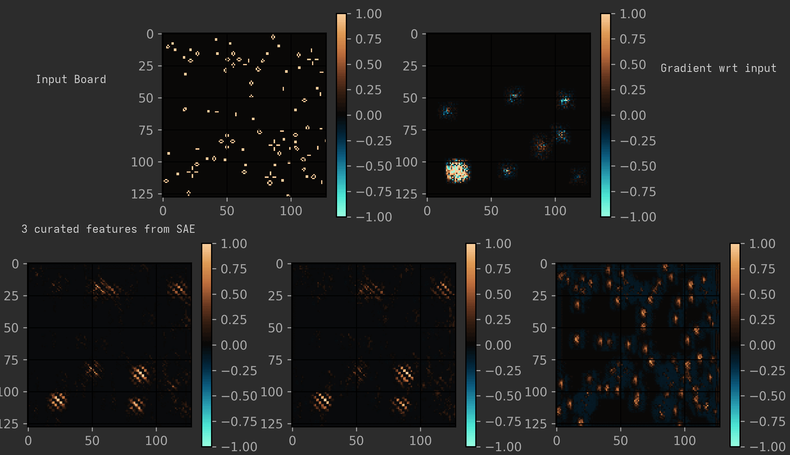
(To visualise it nicely, I have shown the expanded version of the model, as described earlier. Also, the features shown here are three of the cleanest I could find; many features were just messier variants of a ‘traffic light at certain alignment’ detector. Another interesting observation is that it seems to treat honey farms as funny traffic lights.)
But another model I analysed just seemed to have one super-feature that had data of all the traffic lights (and sometimes honey farms too) at all alignments and shifts. And this feature seemed to be so powerful that most of the other features were also just slight variants of that feature. Many of the models had a lot of other minor features that were kind of interpretable, but nothing notable. I also remember seeing features capturing things like vertical blinkers. I only analysed two models here, so take these findings with a grain of salt.
Swap/Ablation Loss
Models resistant to swapping seem to be generally more robust to ablating each individual layer, although not uniformly so. And in most cases, for these swap robust models, swapping adjacent layers does better than ablating either layer, which is suggestive of a common representation between layers, and the importance of every layer.
Many models are much less robust to this. They usually just collapse to 40-50% error on any swap or ablation, which suggests that they follow a more sequential architecture.
| Model | Original Error % | Original-swapped Error % | Expanded-swapped 1 2 Error % | Expanded-swapped 0 1 Error % | 0 ablated Error % | 1 ablated Error % | 2 ablated Error % |
|---|---|---|---|---|---|---|---|
| 3 | 1.8 | 48.7 | 48.7 | 48.7 | 48.7 | 48.7 | 47.6 |
| 11 | 1.5 | 48.7 | 48.7 | 28.6 | 32.9 | 11.8 | 44 |
| 38 | 1.6 | 31.6 | 11.2 | 46.2 | 47.4 | 39.6 | 37.7 |
| 67 | 2.3 | 48.7 | 40.6 | 48.2 | 51.1 | 12 | 48 |
| 84 | 2 | 50.9 | 51 | 44 | 42.5 | 49 | 34.2 |
| 100 | 2 | 48.7 | 46.9 | 48.7 | 48.7 | 45 | 18.4 |
| 102 | 1.8 | 48.7 | 48.7 | 48.7 | 48.7 | 47 | 40.8 |
| 107 | 1.8 | 30.5 | 7.1 | 23.4 | 20 | 36.8 | 36.6 |
| 112 | 1.5 | 47.3 | 15.4 | 17 | 48.7 | 37.1 | 18.8 |
| 117 | 1.6 | 42.5 | 4.2 | 48.6 | 48.7 | 31.5 | 48.6 |
Properties of the weight matrices
The weight matrices broadly seem to be similar. We see highly ill-conditioned matrices and other features on both sides of the spectrum. It is interesting how much variety we see on both sides. Also, the extra training I do before detailed analysis usually increases matrix norms, which is expected as the model becomes more confident in its predictions.
Linear Probing the answer
Linear probing was done on the average value of the activation vector over all the cells. (I also tried taking max, but that completely flopped)
For most models, linear probing gave good results in the last layer, and poor results in the first one. The middle layer showed more interesting behaviour, with two models showing much higher error rates than the other models.
| Model | Original perf | Linear Probe L0 | Linear Probe L1 | Linear Probe L2 | Expanded-swapped 1 2 Error % |
|---|---|---|---|---|---|
| 3 | 1.5 | 16.2 | 4.7 | 3.1 | 48.7 |
| 11 | 1.3 | 16 | 18.2 | 5.7 | 48.7 |
| 38 | 1.5 | 10.3 | 4.3 | 2.4 | 11.2 |
| 67 | 2.1 | 10.8 | 3.4 | 2.6 | 40.6 |
| 84 | 1.6 | 16.2 | 3.2 | 4 | 51 |
| 100 | 2.1 | 10.9 | 4.3 | 3.4 | 46.9 |
| 102 | 1.7 | 13 | 3.6 | 1.6 | 48.7 |
| 107 | 1.6 | 10.2 | 3.8 | 1.9 | 7.1 |
| 112 | 1.1 | 18.4 | 16 | 4.7 | 15.4 |
| 117 | 1.3 | 10.9 | 3.6 | 2.4 | 4.2 |
We can extract a vector from each linear probe’s weights. You could think of this vector as the sort of direction corresponding to the feature of highlifeness. I tried creating a cosine similarity matrix from these to see how common the representations were. This showed some interesting observations, with layers with similar linear probe error rates showing higher similarity, and overall, the cosine similarity tended to be positive. But there were a lot of oddities and exceptions, so it’s best not to come to any conclusions using this.
Hypothesis?
From my experiments, I haven’t really found any better hypothesis than that the model just sometimes randomly decides to either share or not share a common representation of the core features between layers at the critical point, depending on the initialisation.
For the record, my initial hypothesis was that there were two types of models, as classified by their swap loss, which had unique behaviour under other analyses like SAE and linear probes, too. But further testing has convinced me that such relations do not hold, and that most of my initial results were quirks of the specific models I happened to get rather than general phenomena. And that there aren’t two well-seperated classes, but a spectrum.
This also tells us that the model and the problem are complicated enough that two random models vary along several unrelated axes.
Conclusion
From exploring the SAE, my conclusion is that all the models have learnt basically the same thing: the rule is determined by the exact density of traffic lights (and honey farms?) compared to the total density of objects.
It is also interesting how the model seems to focus so much of its effort on traffic lights and has learnt to collapse both TL phases (and honey farms) into one feature. This was unexpected, as I thought it would also use honey farms and highlife constellation as a separate feature, but in hindsight, it makes sense that it would devote so much of its capacity to ensure that no TL, regardless of phase/position/damage, would go undetected.
It seems interesting that there are so many distinct basins of behaviour arising from the exact same training data. I haven’t tried doing this for other models to see if this sort of split is observed even there, so this behaviour may be unique to the idiosyncratic architecture I have been using.
Many aspects of this toy model remain unexplained, like what exactly is the computation occuring at each layer of the model.
I should’ve used a multi-classification task (maybe with B3/S23, B36/S23, B38/S23, B3/S238, etc.) rather than a binary problem. This would’ve made a lot more interpretability techniques accessible and testable.